Cahill 1909
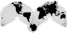
Cahill-Keyes 1975
|
Cahill 1909
|
Go back to Gene Keyes
home page
Cahill-Keyes 1975 |
|
Technical Annexes
Cahill-Keyes Multi-Scale Megamap: Preparing Coastline Data for the Beta-1 and Displaying the Map in Whole or in Part by Gene Keyes
2011-07-01 For fair use, with source credit, by anyone: copy, share, adapt, whatever. (Send me your link!) For commercial use, contact gene.keyes~at~gmail~dot~com |
|
Prologue:
A Do-it-yourself Multi-Scale Megamap
Got some floor-space and time on your hands? And 7,000 sheets of letter-size paper, plus a lot of tape? Or 640 square-meter-size sheets and a wide printer? Or maybe some nice big vinyl media for the gym-size version? There may be a white-elephant factor here; don't remind me. At least we now have the virtual version. Anyone with OpenOffice.org can run it or improve upon it. Or port it to a different program or application. And the virtual Megamap is still worth generating as the source for all its smaller derivatives, partial or entire. And perhaps for all kinds of other GIS content atop its current outline form. And to be a worldwide archetype in lieu of mind-warping maps such as Mercator. Also, a physical Megamap may yet re-enable Buckminster Fuller's World Game, or similar displays.* *In the 1980s, an earlier version of the World Game
had produced a "Big Map": an improvisational patchwork of different map projections
to simulate Fuller's icosahedral, but it was discontinued. Though big indeed,
that floor map was 1/2,000,000, half the scale of the Megamap. See my illustrated commentary about it here and scroll downto Fig. 6.10 ff; see also here:
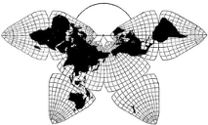
scroll down and to the right. As well, 50 years earlier, B.J.S. Cahill had
drawn up plans for a 1/1,000,000 exhibit of his Butterfly Map in the basement
of the Griffith Planetarium in Los Angeles, but the proposal was shelved. His largest
hand-made prototype was "only" 1/12,500,000.
A 1/1,000,000 globe, DeLorme's "Eartha", is in Yarmouth, Maine. A recent National Geographic program directed by Daniel Beaupré has been renting large floor maps to schools. These are not world maps, but five entirely separate regions (North America; Africa; etc.) only one loaned at a time. They are ca. 26' x 35', with a 10° graticule. RF scales not mentioned. |
| Annex 1: Overview
About Mary Jo Graça's Complementary Programs
"MegamapMaker-prep" (Perl) and "MegamapMaker-plot" (OOo: OpenOffice.org Draw) (Download both in this zip file, 286 KB, expanded.) In previous illustrated postings here, and also here, I have described
my principles and specifications for the Megamap and Cahill-Keyes Octant
Graticule (CKOG) itself, plus its enveloping 40,000 km x 20,000 km grid.
I also described how Mary Jo Graça was able to combine Perl, and OOo
Basic macros, to output an eight-octant CKOG with high precision and a one-degree resolution,
starting at 1/1,000,000.
That brought us to the very difficult next step, which was to draw in the continents and borders, as adapted to the CKOG. It was a task of great complexity, entailing many more weeks of programming. The effort has now resulted in this Beta-1 version of the first entire Cahill-Keyes Multi-Scale Megamap. Just to absorb vector files of coast and border information, three major stages are involved: 1) Acquiring open-source digital geographic data;To elaborate: 1) Acquiring open-source digital geographic data
The complementary
programs function by addressing one octant at a time, because any point on
octant boundaries may correspond to as many as four different x-y coordinates,
on separate octants, due to the map's interrupted shape. Therefore, I needed
my world data in eight installments.
For this early version of the Megamap, I chose a free, readily available, and divisible vector data set from "Coastline Extractor" at NOAA, and downloaded it in eight segments, 90° each of longitude and latitude, corresponding to the eight octants of the Cahill-Keyes. (See Table 1 below.) Living on a retirement shoestring, I was not ready to spend hundreds or thousands of dollars on proprietary CAD and GIS programs. (Besides, the cross-platform OpenOffice.org Draw [OOo] is free.) At first, I selected the Extractor's "World Data Bank II" (WDB 2), suitable for maps up to 1/2,000,000, plus a separate border set. The WDB 2 turned out to have a number of serious flaws, such as an incomplete Japan, badly corrupted Ellesmere Island; missing bits of coastline; excessive clutter of small lakes; and international borders 30 years out of date. Nonetheless, I proceeded for practice to make a first pre-Beta Megamap with WDB 2, on my Asus 701 netbook (and a 19" monitor). An Extractor alternative is the much larger "World Vector Shoreline" (WVS), at a higher resolution suitable for up to 1/250,000. It too has the outdated borders, but avoids WDB's Japan and Ellesmere defects, and lake clutter. The question was whether our little Asus netbooks and OOo could handle such enormous WVS files without choking, as happened on our first two tries. The answer was no. Running WVS's ten-million-point data set overwhelmed my netbook, wrecking its OS, though most of the work had already been done on it. (I can replace the OS; and Mary Jo's Asus netbook survived, since she only composed the program; didn't run it.) Meanwhile, on 2011-04-18, I bought a new 17.3" Acer Aspire 7551-3650 notebook computer, with an AMD Athlon II P340 dual core 2.2 GHz chip, on sale at Walmart for Cdn $448. ("Entry-level", as these things go.) I promptly downloaded OOo 3. Eventually by trial and error and a lot more crashing, we were able to coax it to produce the 40 MB Megamap WVS OOo odg file. (Whereas with WDB 2, the pre-Beta Megamap had been 14 MB, which the netbook could handle — but just barely.) My earlier boast about doing the entire Megamap on the netbooks is still correct — up through the unsatisfactory WDB version. It took the Acer, using the same program, to bring the better WVS coastlines to completion. It may well be that a preferable data set — if I can divvy it into eight octants — is the up-to-the-minute GMT / GSHHS (Generic Mapping Tools / Global Self-consistent, Hierarchical, High-resolution Shoreline Database), which itself is "amalgamated from two data bases in the public domain" (presumably WDB II and WVS ?). Meanwhile, from whatever source, it is necessary that the x-y data be apportioned into the eight Cahill-Keyes octants respectively, with these bounds: Table 1
(Data sets may require positive / negative longitude and latitude, but above are the actual global numbers.) * Octant 2 has so much coastline data that I handled it in three sections: 90-60°, 60-30°, and 30-0°. 2) Converting global longitude-latitude to fit the
Cahill-Keyes framework Mary Jo Graça's 985-line Perl opus, "MegamapMaker-prep" (text in separate window; also in "MegamapMaker.zip"), accomplished the exceedingly difficult feat of converting standard longitude-latitude
digital data to the differentially compressive x-y coordinates
which fit within the eightfold Cahill-Keyes Octant Graticule and Grid spanning 40,000 km by 20,000 km. It revises and extends the earlier version of her program "CKOG-plus". Because the Cahill-Keyes world map transformation is custom-tailored to assure proportional geocells, comparable to a globe throughout the entire map, one cannot use the kind of mathematical formulas of other projections to re-configure digital coordinates (e.g., this is not a gnomonic projection in separate octahedral facets). Instead, the program had to transpose real-world coastline data into the various zones and specified parameters of the Cahill-Keyes Octant Graticule and Grid (See diagrams from link mentioned above.). As I have often mentioned, there is shrinkage toward the center of each octant, but the two outer meridians and equator of each are approximately true to scale of a cognate globe, and the map's overall appearance has good fidelity to any part of a globe. Each of the eight downloaded data files is run through the Perl program, which outputs corresponding text files of x-y coordinates. The input files may be zipped (preferable!) or not. The output file is not zipped. We chose to rename the downloaded files as “oc-#-WVS.zip” and to name the output files as “xy-#”, where # is the octant number. Perl, being a script language, does not need to be compiled, but the program’s permissions must allow execution. These eight large reprocessed Cahill-Keyes x-y coordinate data files are then used by the complementary program, "MegamapMaker-plot", a complex of macros in OOo Draw 3, which outputs the vector image: graticule and grid; coastlines and borders: the whole earth in a single conspectus. The file tops out at 40 MB in its 1/1,000,000 master version, an enormous graphic of the entire Beta-1 Multi-scale Megamap. In addition, it may be possible to connect the Perl "MegamapMaker-prep", and/or the Cahill-Keyes x-y data files, to other CAD, graphic, or GIS programs. (We had initially linked the Perl to an outdated version of TurboCAD, before discarding it in favor of OOo.) Also, numerous comments have been included in the Perl script, should one wish to adapt it to a different programming language. (User interface for running this Perl is further described in Annex 2 below.) |
|
3) Plotting the Megamap itself
MegamapMaker-plot is an OpenOffice.org Draw document (odg),
comprising five separate pages within the same file. Thumbnails of these
pages are in a column to the left of the currently-chosen page. (See screenshot, Fig. 5, near end of this page.)
p.1, “Read-me”, shows where to increase the graphics cache size for its immense output, a 40 MB document. With such a long plotting time, in earlier runs we could not tell whether OOo was working, or had stalled somewhere. We therefore programmed the plotter to show constant updates as to number of lines and segments drawn thus far, and "beeps" to indicate the map is in progress. As well, once the complete map has been successfully plotted, its land masses still cannot be seen on a monitor, because of the Megamap's enormity, covering a potential floor space of 800 square meters (ca. 957 square yards, or ca. 8,611 square feet). OOo's maximum image-reduction onscreen is to 5%, but even that depicts mostly empty background space or ocean, not the continents. Therefore — besides getting data, converting it, and plotting it — three other steps were still required to make this macroscopic map visible on an ordinary monitor, be it desktop, laptop, or even netbook; as well as in hard copy for notebook, textbook, atlas, or various wall-map sizes, in addition to the showpiece parent Megamap. Reprising how we did this with macro-linked buttons (and pardon my redundancy): 4) To re-scale the maps: I make eight separate files, duplicating, at first, the Megamap file itself. The "Resize Main Frame" is then used to reduce them respectively to the progressively smaller scales listed in Table 2 below, each in a 2 x 1 ratio (the "double-square", as mentioned at Fig. 1 on previous page). Despite their smaller sizes, their content is identical to the Megamap original, and all scales retain a full one-degree graticule!(User interface for running this plotter is further described in Annex 3 below.) |
|
Next are some screen shots showing how the macro-activating buttons work.
They are the only ones included in the Megamap odg file itself, (The others
from MegamapMaker-plot are in Fig. 5 further below.)
|
|
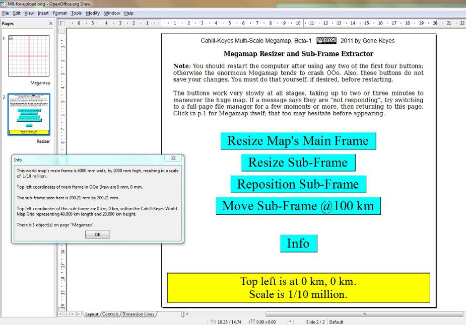
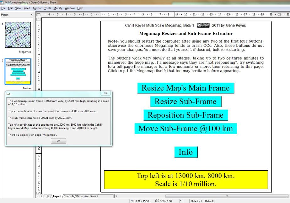
Fig. 1:
This shows the five buttons in the given Sub-Frame, at its default size of
200 mm x 200 mm. The buttons are in p.2 (thumbnails at left), and the map
Sub-Frame is in p.1. (These images are not made from OOo, but a separate
screen-shot tool for that, depending on which computer OS you use.)
Here I have already resized the Megamap to 10 times smaller, at 1/10,000,000, changing its length to 4,000 mm from 40,000, by means of the "Resize Main Frame" button. Because the upper left corner remains at its 0,0 origin, the frame is still almost empty, except for the “Read-me” from the Megamap itself, legible when the map is ten times larger at Scale 8, namely, 1/1,000,000. (Review the “Read-me” jpeg, in Fig. 14, previous page, for what happens when the Megamap is reduced to 1/200,000,000.) I have also clicked the "Info" button, which yields a pop-up box, with additional numbers, besides those in the larger yellow text frame. |
|
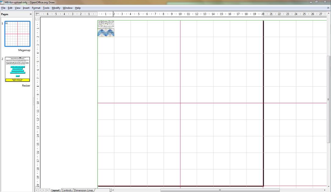
Fig. 2: Now I have clicked in the p.1 thumbnail to show the full-size frame, as yet
mostly empty, except for the grid, and the shrunken Read-me.
Note: the Acer’s onscreen images, whether odg, pdf,
or jpegs, are too large, perhaps due to my settings in Windows 7, an OS which
I do not normally use. (Their print size is correct.) Meanwhile, I reduce
the Acer’s jpegs, when composing this Web page on my old Mac OS 9 and 19”
monitor. But the scale can vary from one monitor or platform to the next,
as I constantly reiterate on the previous page. |
|
|
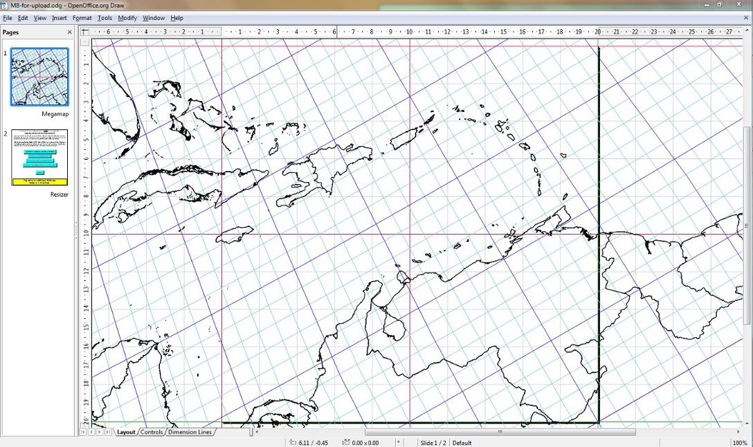
Fig. 3: Next,
I have focused on the Caribbean (for Fig. 6 on previous page), using button
"Reposition Sub-Frame", and changing the upper left km coordinates from 0,0
to "130,80" (in hundreds of kilometers: i.e., 13000,8000 as shown in the
information boxes). Now we see an actual map in the p.1 thumbnail, and will
see its actual size when we click in that thumbnail (Fig. 4 below.)
For this image, I have again clicked the “Info” button, to show its pop-up box. Note: The Main Frame coordinates listed there are negative because the program moves the map itself, not the Sub-Frame. (Took me a while to comprehend that; Mary Jo had to explain it several times...) Those figures are not of concern to the user; it is the Sub-Frame km coordinates which one enters to call out a given segment. When a Sub-Frame map coincides with a Main Frame map as a whole-earth view, they both have an upper left origin of 0,0. |
|
|
Fig. 4: Here we switch from button page to map page (via thumbnails). The default Sub-Frame
size of 200.21 mm x 200.21 mm is indicated by OOo's darker "shadow" lines
at bottom and right, which is how OOo Draw works. Your own eyes have to fill
in the top and left sides.
Note: only the Sub-Frame is shown in the left-hand thumbnail. It is only that portion which will be printed by OOo or exported to a pdf or jpeg, not the rest of the map on this screen. Otherwise, you must specify a larger Sub-Frame with the second button. |
|
|
Although these buttons are ingenious, and indispensable to the Megamap and
its progeny, at this Beta-1 stage they are slow and inefficient
in the absence of direct panning, and slider scaling. Perhaps such functions
will be developed in later Beta's, or by other Megamap users.
It also seems that because the map is so humongous, even the new Acer can only do about two of those button operations on the map at a time, before it needs to be restarted; otherwise OOo crashes. I'm still learning the Acer-OOo nuances and "Simon-says's" as I go. For example, as mentioned, unlike OpenOffice.org 2 on Asus, OOo 3 on Acer requires an extra 0.21 mm on its frame dimensions to avoid trimming off the bottom and right grid lines. It took a lot of trial and error to nail that one down. Anything less omits some grid lines; anything more overshoots them. Another nuance is that these giant odg files at almost every step give a transient spinning-wheel and message "Program not responding." Again, by trial and error, we found that we could either wait it out for a few moments, or often alleviate that condition by switching to a full-screen directory (file manager), then returning to OOo after a pause of up to a minute or so. Usually it is a false alarm. But if we have over-used the buttons without re-starting, then that spinning wheel is likely to turn into a crash.
Scales
The above buttons enable the Cahill-Keyes Megamap
to be adjusted both for screen display and actual or potential printout,
in my preferred sequence of eight scales. All of them are size / scale reductions
of that selfsame original 1/1,000,000 Megamap, and so, to repeat, all of them have a one-degree graticule.
Any other scale is possible here — including larger! — , but my defined set has always increased from the small Scale 1 (1/200,000,000) @ 2x, 2x, 2.5x. My Coherent World Map System is especially concerned about counteracting the random, chaotic, and unbalanced scales found in most atlases and historical atlases. Table 2
|
|
ANNEX 2:
User interface for generating Cahill-Keyes x-y coordinates
via “MegamapMaker-prep” in a Linux shell terminal:
(Note: I am now returning to the first program, to describe in more detail the steps involved in running it.) The first part of the MegamapMaker pair is
executed in Perl, assuming your computer has Perl to do so. (Linux already
includes it; or you can download Perl from the Web for other platforms; a freebie.)
Table 3: Lines of data and plotting time for the 8 octants respectively:Let us suppose that you have downloaded eight zip files of x-y coastline data, e.g., from Coastline Extractor, aligned to the eight Cahill-Keyes octants, in MAPGEN format, according to the longitudes-latitudes in Table 1 above. For a Unix or Linux system, be sure that the program "MegamapMaker-prep" has execute permission. Run it, likely in a terminal window, by entering: ./MegamapMaker-prep and then the return key. [The revised program lists five options about generating the Cahill-Keyes octant and graticule; here we are only concerned with coastline and border data. Therefore enter the number 1, then return.] Whereupon it asks the user, “For which octant do you want to prepare data (1 to 8)?” User enters number, and return. Program says “Type in name of MAPGEN file with coastal data.” User types in, e.g., “oc-1-WVS.zip”, and return. Program says “Type in name for output file to receive x,y coordinates.” User types in, e.g., “xy-1”. (When we were doing separate WDB files for coastline and border respectively, output files were named “xy-1-c” (for coast) and “xy-1-b” (for borders). But with WVS, we are using a file which combines both Program announces “This might take awhile. I’ll let you know every 1,000 lines that I read.”; then it lists them quickly while in progress, ending at different totals for each octant, ranging from over 232,000 lines for Octant 8, to almost 3,000,000 lines for Octant 2. (A line of data is a new segment indicator or a longitude-latitude pair. A segment is a cluster of data lines. Note that the program states how many lines it has read, but not how many it wrote, because it omits any consecutive repeated lines.) To prepare the other octants, proceed as above, with different input and output file names. You now have a set of eight large xy text files (actually, ten, because we split Octant 2 into three parts). These go into the same folder as "MegamapMaker-plot". In the downloadable zip file, I have already named that folder "MegamapMaker"; it contains both the ...prep and ...plot programs, plus an essential text file called "OctantTemplate.txt", and will contain the xy files which you create with ...prep. Table 3 below lists lines of data of the MAPGEN files for the respective octants. (The actual total as plotted is somewhat less than the input lines, because, as mentioned, consecutive identical ones are omitted.) The grand total is over 10,000,000. (Of interest here are mainly orders of magnitude: Octant 2 includes all those Arctic islands, besides much of North and South America, while Octant 8 only has the southern one-fourth of Africa, and Octant 6 has New Zealand and mostly Pacific Ocean.)
*Net
plotting time per single octant. In addition, each one requires some extra
time, averaging ca. 15 minutes, for loading the file, grouping its objects
and saving it as part of the macro process, then restarting the computer.
Thus. approximate total for plotting a WVS Megamap (on my Acer 7551) is 361
minutes, or ca. 6 hours, + ca. 2.5 extra hours, for elapsed time of ca. 8.5 hours.
|
|
ANNEX 3:
User interface for plotting Cahill-Keyes Megamap via
"MegamapMaker-plot" in OOo Draw 3 (or 2) (see Fig. 5 below) After much trial, error, and crashing, we found
it was best to plot the Megamap one octant at a time, then restart the computer
before going on to the next. (Earlier, we had tried to plot everything in
one go.) As well, we found it best to start with the octants having smallest
number of lines, and end with the largest.
The prep
xy files which the Perl program generates go in the same folder as, and will be read
by, the other program, "MegamapMaker-plot". (The zip file of these two programs, plus a third requisite text file,
come already put into a folder "MegamapMaker", to which you will also direct
your converted xy-files.) This runs a number of macros in OOo Draw, to produce the Megamap in all its immensity at 1/l,000,000.
First, after opening the "MegamapMaker" folder, you click the OOo "MegamapMaker-plot" icon, which, when loaded, will ask you to enable its macros. Click yes. Whereupon it opens the five-page OOo Draw program described above. whose initial button, on p.2, "Plot Grid and Graticule" sets the procedure in motion. It does just that in about two minutes (on the Acer Notebook). The next button, "Plot Coastline and Borders", asks you what xy-file to use; here you enter the name of one of them, starting, as mentioned, with the smallest, xy-8 (Table 3 above). Grouping, and then saving, are part of the macro process for each octant, and when that is done, you restart the computer before going on to the next octant. When all the octants are finished, then after restarting you click on the "Group Map" button, which takes awhile to consolidate the many separately plotted components. Meanwhile, there is no need to look at the Megamap image on p. 5 because there is nothing to see until the map size has been reduced, or an extract selected. The cumulating Megamap file will save itself under its original name, "MegamapMaker-plot.odg" Afterward, I renamed it M8.odg, for Scale 8 (1/1,000,000). The physical length of this 40 mb file is 40 meters (i.e., 40,000 mm). I then made seven duplicates of it, renaming them M1 through M7. (Besides backups backups backups of course.) To make the next smaller scale, 1/2,000,000, I opened the M7 odg file, still at 1/1,000,000, and used the "Resize Map's Main Frame" button, on p.4 to do just that: change its main frame length to 20,000 mm, then saving the file. Half the original length of the Megamap results in half the scale. I did similar changes for the remaining six scales. (See Table 2 above. Length must be twice the height; the latter is automatically adjusted by the macro.) To generate sub-maps of continents, regions, countries, etc., at whatever chosen scale, you should make duplicate files of the Megamap and/or one of its junior versions. You then discern where to locate the upper left corner of a Sub-frame, and enter its x-y km coordinates in the dialog box of the "Reposition Sub-Frame" button. Note: As of Beta-1, these buttons are quite slow to respond; and to execute. You need patience, and also to remember to restart the computer after no more than two button commands, lest it crash. (All this is in terms of my new Acer; specs mentioned above.) For instance, to make an odg, jpeg, or pdf of, say, Hispaniola and vicinity, as in Figs. 3 and 4 above, you first load an entire world map of say, 1,10,000,000, Scale 5, (that takes awhile); then if required, use the "Resize Sub-Frame" button (that takes awhile); then set the "Reposition Sub-Frame" coordinates in hundreds of km — in this case, 130,80 — (that takes awhile); then "export as" one of those formats (that takes awhile; the computer may hesitate for up to several minutes before responding to each of its own three-step export clicks). Then, before doing another Sub-Frame, you close the program, and if you save it as a particular file, that takes awhile. Then you restart the computer, and reload another Megamap. That takes awhile... All this digital foot-dragging is because — even at the smaller scales — the program has the whole wide world in its hands. With every move, it is lugging over ten million data points. There may be more efficient ways to go about it, but that's why this is a Beta-1. |
|
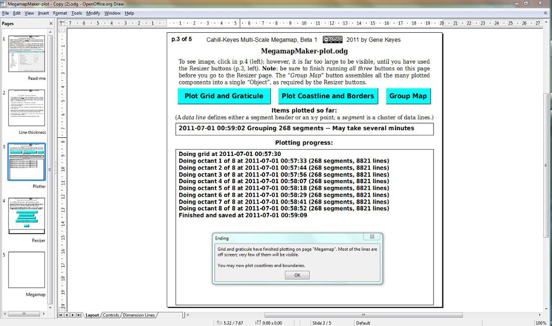
^ Fig. 5: Here is a screenshot of the plotting
buttons. (The resizer buttons are shown above in Figs. 1 and 3.) For this
picture, I have already plotted the grid and graticule, to show the progress messages.
Note: the 117 KB "MegamapMaker-plot" file has five pages, as seen here, including the resizer buttons, but the 40 MB "Cahill-Keyes-Megamap.odg" file only has two pages: the pre-drawn map itself, plus the resizer buttons. |
|
|
Epilogue
Meanwhile, I'll continue to experiment
with the Megamap:
formats and excerpts; numbering and lettering; geopolitical and historical overlays, etc., while hoping for an user-base to enrich its content and simplify its procedures. And some patrons to produce and host an exhibition-size Megamap? |
|
Questions, comments, problems, bugs: contact gene.keyes at gmail dot com.
|